Interpolation and Curve Fitting

Why would we need to approximate a function/fit a curve?

An integral part of computational economics (and numerical methods in general) is using appropriate approximation techniques. Computational methods are attempts to approximate something to a high degree of accuracy. We will discuss several types of approximation that are normally used: Local Approximation, Orthogonal Polynomials, Regression, and Interpolation but there are many others that can be used. For more information refer to Kenn Judd’s “Numerical Methods in Economics” [Judd1998].

Local Approximation

Local approximation is an approximation technique that is centered at a point \(x_0\) and requires a certain information about the function, \(f\), at this \(x_0\). Typically this information includes the value of the function at \(x_0\), along with needing to know several derivatives of \(f\) at \(x_0\). A form of local approximation is Taylor Series, where one represents the function \(f(x)\) as \(f(x) = \sum_{i=1}^{\infty} f^{(n)}(x_0) \frac{(x-x_0)^n}{n!}\). Since most of you are familiar with Taylor Series, and since tangent lines aren’t particularly interesting, we are going to focus on something known as Pade Approximation.

Pade Approximation

A \((m,n)\) Pade approximation of \(f\) at \(x_0\) is a rational function \(r(x) = \frac{p(x)}{q(x)}\) where \(p(x), q(x)\) are polynomials, the degree of \(p\) is at most m, the degree of \(q\) is at most n, and \(0=\frac{\partial^k}{\partial x^k}(p - fq)(x_0)\), where \(k \in 0, 1, 2, ..., m+n\).

In Pade approximation one usually chooses \(m=n\) or \(m = n+1\). This allows the defining conditions to be rewritten as \(q(x_0) = 1\) and \(p^{(k)}(x_0) = (fq)^{k}(x_0), k = 0, 1, 2, ..., m+n\). The conditions on the coefficients will give us \(m+n+1\) conditions and to get the last condition (since there are m+n+2 coefficients), we choose to normalize \(q(x_0)=1\).

In the practice one typically replaces \(f\) in the above equation with its taylor approximation out to \(m+n\) degrees. Then you can solve the equation \(p(x) - f(x)q(x) = 0\). This facilitates solving the equation. Since for all possible \(x\) the equation must be equal to 0, you can set the coefficients of each order of \(x\) equal to 0. I would suggest reading more on wolframalpha or padeproof.

Todo

You have two options; either work out by hand the (3, 2) Pade approximation centered at 1 of the function \(x^{\frac{1}{4}}\) or create a general python function that relies on sympy that will create a Pade approximation. The Pade function should take as an input the following: A function, a list or tuple with the degree of approximation (m,n), and a point to center the approximation.

Todo

Create and compare the Pade approximation, tangent line, and 5th order taylor polynomial all centered at 1 of \(x^{\frac{1}{4}}\). After working them out, create a table to compare their accuracy from .5 to 3 in .5 intervals. Should look something like:

Errors from different local approximation techniques
Value	Tangent Line	Taylor Polynomial	Pade Approximation
.5
1
1.5 (etc)

Orthogonal Polynomials

While it is natural to think of the span of continuous nth order functions to be the monomials \(1,x,x^2,...,x^n\), a better basis would be orthogonal or better yet orthonormal.

Weighting Function, w(x):

A weighting function, \(w(x)\), on \([a,b]\) is any function that is positive almost everywhere and has a finite integral on \([a,b]\).[Judd1998]_

Given \(w(x)\), we let the inner product be defined as: \(<f,g> = \int_a^b f(x)g(x)w(x)dx\). Then a family of polynomials, \({\Phi_n(x)}\) is orthogonal if \(\forall n \neq m, <\Phi_n(x), \Phi_m(x)> = 0\) and orthonormal if it is orthogonal and \(<\Phi_n(x), \Phi_n(x)> = 1\).

There are many types of orthogonal polynomials: Legendre, Chebyshev, Laguerre, Hermite, etc... We will briefly discuss Chebyshev polynomial approximation.

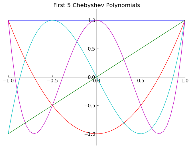
Chebyshev polynomials can be built in several ways, but we will use the following recursive method. Let \(T_{i+1}(x)=2xT_i(x) - T_{i-1}\) and \(T_0(x)=1, T_1(x)=x\) where \(T_{i+1}\) is the i+1th order Chebyshev polynomial.

In [1]: plt.show()

Todo

Write a short python function that will calculate the first n Chebyshev polynomials. Then call this function to plot the first 7 Chebyshev polynomials (pretty plots would be nice, but not required... Plotting lab is next week; maybe you will have to redo it).

Note

Hint for the homework. Your function should create a list of functions. It may be helpful to have cases for \(n=0;n=1;n>1\). Will need to call functions recursively and would suggest using the np.vectorize(function). Here is a skeleton for your code: chebyshevfunc.py

Regression

This is one of the most commonly used forms of approximation. Many of us are familiar with regression through statistical applications. The most common type of regression is least-squares regression in which one fits a line (usually linear although there is non-linear least-squares methods as well). In regression one takes m facts to fix n parameters where \(m>n\). This will typically be used in an econometric framework for several reasons. For example: An econometrician in unable to choose the \(x^i\) that he uses in his regression, but numerical methods usually allow you the ability to choose your \(x^i\).

This will be a quick review of Least Squares. Given a set of points/data \((x,y)\), we can approximate the relation between \(x\) and \(y\) by setting up a linear system \(x \beta = y\). Suppose \(x \beta = y\) is an inconsistent linear system of \(m\) equations and \(n\) unknowns where \(m>n\). Then the errors(inconsistencies) of our linear system can be expressed as \(x \beta -y=e\) where \(e\) is the error vector. The goal of least squares is to minimize the \(e^2\). To minimize \(e'e\) we proceed in the following fashion.

\[e'e = (y - x \beta)' (y - x \beta)\]\[(y - x \beta)' (y - x \beta) = y'y - \beta' x' y - y' x \beta + \beta' x' x \beta\]\[\text{since each of these terms are scalars and for any scalar c' = c,}\]\[\text{then we can tranpose the middle terms to make them the same thus }\]\[y'y - \beta' x' y - y' x \beta + \beta' x' x \beta = y'y - 2\beta' x' y + \beta' x' x \beta\]\[\text{ We want to minimize with respect to } \beta\]\[(y'y - 2\beta' x' y + \beta' x' x \beta) \partial \beta = 0 - 2 x' y + 2 x' x \beta = 0\]\[\rightarrow x' y = x' x \beta \rightarrow (x' x)^{-1} x' y = \beta\]

Thus we see that the minimizing solution to \(y - x \beta\) is \((x' x)^{-1} x' y = \beta\).

Todo

Using the data in regdata.csv, use a least squares method to fit two curves to this data (Note that the data is in two columns, the first one is x and the second is y):

1. A standard cubic polynomial in x: \(a_0 + a_1 x + a_2 x^2 + a_3 x^3\)
2. A 3rd order Chebyshev polynomial in x :\(b_0 + b_1 T_1(x) + b_2 T_2(x) + b_3 T_3(x)\)

Plot the original data as well as your two fits on the same axis. When plotting use the original x data as the input to your fit. Also return the mean error for each method.

Interpolation

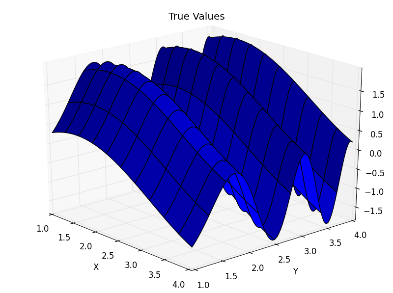
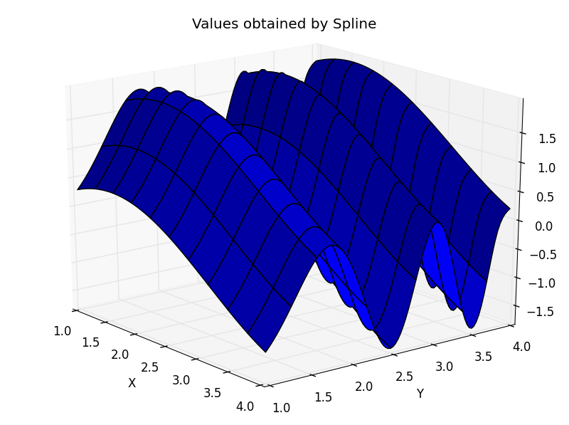
Interpolation is another form of curve fitting. Specifically, given a set of points, \((x_n, y_n)\), on the interval, \([a,b]\), where \(x_0=a; x_n=b\), interpolation generates a “nice” function that can generate new points on the specified interval. Normally interpolation only maintains accuracy if you are on that interval; once you leave the interval it is unlikely that will continue to successfully approximate the function (One can read more about this error on page 220 of [Judd1998]). Accuracy is also dependent on the number of nodes (evaluated points you start with) that you choose. Below on the left is an example of the function \(sin(x) - cos(y^2)\) and on the right is an interpolated approximation (using cubic spline; n=45).

There are many different kinds of interpolants: Linear, orthogonal polynomial, nearest, splines etc... Each of them have different applications and can be used for different things. In your homework problem, you will experiment with several different types and compare their errors.

Todo

Using the scipy.interpolate.interp1d function analyze the average absolute error \(\sum_{n=0}^N |error|/N\) obtained in interpolation on the interval \([-4,4]\) (except on \(x^{1.4}\). Use the interval .5 to 3 on that one.) using nearest, linear, and cubic interpolation for the following functions: \(f(x) = \frac{2}{x-3}, x - 2, x^3 -8x + 2, x^{1/4}, \frac{1}{x}cos(x)\) with \(n=5, 10, 50, 500\). Additionally, graph the true values and interpolated values of the functions. What do you observe? Which performs best for each of the functions? How much of a difference is there in the number of nodes you use? Is extra computation time worth the improvement in accuracy? Is there something you can learn from this? Put your error values in a table similar to the one below. How do the errors for \(x^\frac{1}{4}\) compare to the local approximations? You will turn in four tables; one for each number of nodes.

Hint: make sure your x data doesn’t ever equal exactly 3 when fitting the first function and 0 when fitting the last function. If you create equally spaced data on the given interval using the number of points given you won’t have a problem, but it is a good sanity check to look at your x data.

Errors from different interpolation techniques with n nodes
Function	Nearest Interp	Linear Interp	Cubic Interp
\(\frac{2}{x-3}\)
\(x - 2\)
\(x^3-8x+2\)
\(x^{1/4}\)
\(\frac{1}{x}cos(x)\)

B-Splines

Motivation

One common type of function that comes from numerical analysis is the B-spline. B-splines are smooth, piecewise functions exhibit many desirable mathematical properties.

• B-spline functions have a high degree of smoothness where the functions come together (called knots)
• B-spline basis functions have a compact support
• B-spline basis functions are a partition of unity
• B-spline functions are \(C^{\infty}\) in between knots and \(C^{p-k}\) at knots, where \(p\) and \(k\) are the degree the spline and multiplicity of knot, respectively.

Because of this flexibility, B-splines are used in many different fields in order to achieve different things. For example, when you watch a Disney-Pixar movie, you are really just watching a bunch of B-splines moving around and interacting on the screen. In scientific applications B-splines are often used for many different purposes. Among these applications are signal analysis, design specifications in CAD programs, image processing, and our application: function approximation.

The following was taken from the seminal resource on splines:

A fundamental theorem states that every spline function of a given degree, smoothness, and domain partition, can be uniquely represented as a linear combination of B-splines of that same degree and smoothness, and over that same partition. – Carl DeBoor [DeBoor2001]

Some terms in the above statement may not be clear to the reader who hasn’t studied splines before, but it evident that B-splines are very flexible and powerful modeling tools. For this reason we will be teaching some basic theory behind how B-splines are formed as well as explaining how to implement them in code.

Theory

We will be interested in using B-splines for function approximation and interpolation. The technical term for this type of B-spline is a B-spline curve. In order to construct a B-spline curve, we need 4 things:

1. A set of knots
2. A set of basis functions
3. A set of control points
4. A set of coefficients

I will provide a high-level example of what those four items are and then we will dive into the more detailed explanation of how to create and use them.

First Example

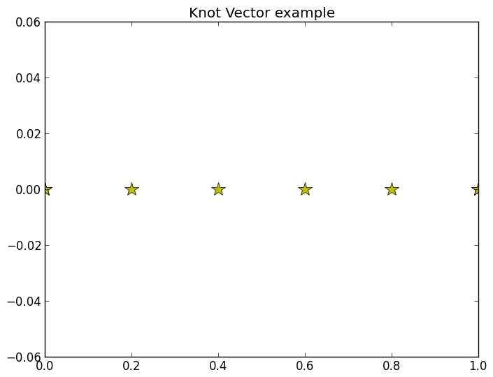
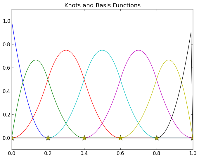
Knots are the points at which the B-spline basis functions are joined together. The location and multiplicity of the knots control the continuity of the spline at these junctions. We will call the knots \(u_i\) and we will say that there range from \(i=0\) to \(i=m\) and that they are non-decreasing in their index. The set of the \(m+1\) knots \((u_0, u_1, \dots, u_m)\) is known as the knot vector and is given the name \(U\). The knot vector is specified when the B-spline is first created, but can be altered later via various knot insertion algorithms. The knot vector might look like the yellow stars in the plot below.

In [2]: knots = np.array([0, 0, 0, .2, .4, .6, .8, 1, 1, 1])

In [3]: fig, ax = plt.subplots(1, 1)

In [4]: ax.set_title('Knot Vector example')
Out[4]: <matplotlib.text.Text at 0x1108c8b10>

In [5]: ax.plot(knots, np.zeros_like(knots), 'y*', label='knots', markersize=15)
Out[5]: [<matplotlib.lines.Line2D at 0x1108cd950>]

The basis functions of a B-spline are rigidly defined from a degree parameter \(p\) and a knot vector. \(p\) is simply the degree of the individual polynomials used to create the B-spline. See the constructing basis functions section below for more information on how this basis is defined. For now we will simply add the basis functions for the know vector above and \(p=2\) (quadratic basis functions) to the plot from above. (Note that the code used to generate the plots is hidden because constructing the basis functions will be an assignment)

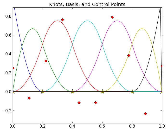
In a curve fitting context, the control points are the data points or observations you want to fit a curve to. We will represent them with red diamonds and add them to the plot below.

# Just making up x, y data
In [6]: control_x = np.linspace(0, 1, knots.size)

In [7]: control_y = 0.5 * np.random.randn(knots.size)

In [8]: ax.set_title('Knots, Basis, and Control Points')
Out[8]: <matplotlib.text.Text at 0x1108c8b10>

In [9]: ax.set_ylim(control_y.min() - .1, control_y.max() + .1)
Out[9]: (-0.33473719296747606, 0.8896064077536957)

In [10]: ax.plot(control_x, control_y, 'rD', label='Control')
Out[10]: [<matplotlib.lines.Line2D at 0x1108de910>]

Finally, the coefficients of a B-spline curve are simply real numbers that connect the basis functions to the data. Some ways to obtain these coefficients would be to use regression methods, collocation methods, or solving linear system. Regression techniques are the most familiar to an economist, so that is was we will use in this tutorial. We will cover this in more detail later.

Constructing the B-Spline

The first step in using a B-spline to construct an interpolator is to define the knot vector and the basis functions for the spline. There are various algorithms that can be used to define these items, but we will cover the simplest cases here: a clamped uniform knot vector and the Cox DeBoor recursion algorithm to define basis functions.

Defining the Knot Vector

The knot vector can be defined in almost any way, with the only restriction being that the knots are ordered in a non-decreasing manner. However, there are various algorithms that produce knot vectors that lead to more robust and accurate interpolators. Among these algorithms are the uniform method, chord length method, the centripetal method, and the universal method. Each of these methods has a number of variations that affect the behavior of the spline at the end points and continuity at knot junctions (for more information on the various algorithms as well as the differences in the variations see these websites: 1, 2). For our purposes, we will be using a slight variation of the uniform method to generate a clamped B-Spline. The fact that our splines are clamped simply leads to the interpolator being exactly equal to the data at the end points.

Formally, the uniform method for knot vector depends on the number of control points. This is great when creating a spline only to be used with a particular data-set, but we would like to define our splines independent from the data. To do this we will need to select a parameter \(n\), where \(n+1\) is the number of data points (I represent it this way to follow conventions defined in other resources on Splines) and the degree of the underlying basis functions \(p\). Once \(n\) and \(p\) have been chosen, the algorithm for generating a uniformly spaced knot vector on the interval from \([a, b]\) is simple:

\[u_0 = u_1 = \dots = u_p = a\]\[u_{j + p} = a + \frac{j}{n - p + 1} (b - a) \quad \text{for } j = 1, 2, \dots, n - p\]\[u_{n-p} = u_{m - p + 1} = \dots = u_{n} = b\]

This will result in a total of \(m+1\) knots where \(m = n + p + 1\). Again, I use the parameters \(m, p\), and \(n\) to be consistent with the standard notation.

Todo

Write a function that will take parameters \(n\), \(p\), and domain = (a, b) and compute the \(m+1\) uniformly spaced knot vectors.

Todo

After ensuring that your function from the previous problem works, implement its logic within the _create_knots method in the BSplineBasis class in the (downloadable) file bspline.py. HINT: the function signature is _create_knots(self, n, method='uniform'). Notice that there is no place to input the parameter p. Following the note below you see that you can actually access this parameter inside the _create_knots function using the name self.degree. This means that you might want to put the line p = self.degree somewhere towards the beginning of your implementation of _create_knots. Also, for now don’t worry about the code related to how or the specification how=uniform. It is simply a placeholder to remind us that we might want to allow for more flexibility in knot vector creation in the future.

Note

Using the class keyword is an example of object oriented programming (OOP). We have not covered OOP yet, but we will towards the end of bootcamp. A word is in order regarding the self keyword that is used in a class definition. self simply refers to the particular instance of the class that is being created, called, or accessed. The way you attach instance variables (data) to a class instance is by to set the parameter using the syntax self.param = value. Then, inside another method (function) in the class definition you can access that data with the syntax value = self.param. If wanted to access these instance variables or a class’s methods from the python interpreter you simply access them with object_name.param. For example, assuming you have a numpy array named x, you would access the shape instance variable via x.shape. ALSO note that functions with two leading and trailing underscores (like __init__ and __call__) are special “overloaded” functions that python treats a bit differently than other functions. We will discuss the details more later in bootcamp.

Defining the Basis Functions

Given a set of \(m+1\) non-decreasing knots \(\{u_i\}_{i=0}^m\) and a non-negative degree \(p\), we can define the set of basis functions \(N_{i, p}(u)\), where \(i\), \(p\), and \(u\) represent the number of basis function (to keep track of them), degree of underlying polynomial, and location the basis function should be evaluated at, respectively. The definition of these functions is recursive as defined below.

\[\begin{split}N_{i, 0}(u) = \begin{cases} 1 & \text{if } u_i \leq u < u_{i+1} \\ 0 & \text{otherwise } \end{cases}\end{split}\]\[N_{i, p}(u) = \frac{u - u_i}{u_{i+p} - u_i} N_{i, p-1}(u) + \frac{u_{i + p + 1} - u}{u_{i+p+1} - u_{i+1}} N_{i+1, p-1}(u)\]

This recursion might look difficult and a bit intimidating, but it is actually quite simple. Notice that when \(p=0\), the basis functions are all just step functions that turn on and off depending on the location of \(u\) relative to the knots. Also notice that for \(p>0\), two of the \(p-1\) basis functions are needed. So, when constructing the basis functions of degree \(p\), you will need to use basis functions for every order between \(0\) and \(p-1\).

Looking at the recursive part of the above algorithm you notice that there is potential for dividing by zero. This will happen whenever there is a knot with a multiplicity of \(p\) or greater. In order to overcome this in computation, the person coding this algorithm should check to make sure that the two terms in each denominator are not equal. If the knots are equal, the entire term for which the denominator would be zero should be set to zero.

A few important properties about these basis functions are given below:

• \(N_{i, p}(u)\) is a polynomial of degree \(p\) in \(u\).
• Non-negativity: \(N_{i, p}(u) \ge 0 \quad \forall p, q\)
• Local-support: \(N_{i, p}(u)\) is non-zero only on the interval \([u_i, u_{i + p + 1})\)
• Partition of unity: On the interval \([u_i, u_{i+1})\), \(\sum_i N_{i, p}(u) = 1 \quad \forall i, p, u\)
• At a knot of multiplicity \(k\), the basis function \(N_{i, p}(u)\) is \(C^{p-k}\) continuous.

Todo

Keeping these points in mind and referring to resources like this site or this wikipedia article fill in the _create_basis method in the BSplineBasis class you worked on earlier.

Todo

Implement the __call__ method in BsplineBasis that will evaluate the basis functions for a given index (index is the \(i\) in \(N_{i, p}\)) or for all the basis functions for a given vector of \(u\) data. HINT: The docstring for this function should give you an idea of how to structure the function. Also, in order for the __call__ method to work for an entire array of input data, you will need to have followed the hint about np.vectorize in the docstring of _create_basis.

Looking at the file bspline.py you will notice that I have filled in two other methods for the BSplineBasis class: __init__ and plot_basis. The __init__ method is what actually creates an instance of our class when the class is called. This is where instance variables like degree and funcs are attached to an instance of the class. plot_basis is simply a utility method that can be used to quickly generate a plot of the basis functions and knot vector. I will demonstrate how you might want to verify that your code is correct below.

# Create the instance of our BSplineBasis class
basis = BSplineBasis(2)

# Create x array to test evaluation
x = np.linspace(0, 1, 200)

# Use __call__ method to eval 1st and 2nd basis funcs at x
y_0 = basis(x, index=0)
y_1 = basis(x, index=1)

# A 2d array. Uses __call__ to eval all basis funcs at x
all_y = basis(x, 'all')

# Generate plot of basis funcs, should look like my plot above
basis.plot_basis(ion=True)

Constructing a B-spline curve (interpolating)

Once the basis functions have been defined and the control points (data) have been collected, the next step in using B-splines to interpolate is to determine values of coefficients. Just like there are many algorithms for computing an optimal knot vector, there are many ways to extract the coefficients that unite a B-spline basis with a data set to form an interpolator. Some of these ways are somewhat complicated and require the user to define knots, basis functions, and other parameters based on the actual data to be used. Others are quite simple and can be used to quickly generate a B-spline representation of a data set. We will be using a simple least squares regression method, but it should be noted that for maximal accuracy and efficiency, other methods should be considered.

Setting up the Problem

Before we get started, let’s review what we need to have defined in order to proceed:

• A set of \((x, y)\) data. Define \(\theta\) as the number of data points
• A degree parameter \(p\) specifying the degree of polynomials in the basis functions
• A parameter \(n\) used to determine the number of knots
• A knot vector of length \(m+1\) (\(m = n + p + 1\))
• A set of \(n-p\) basis functions \(N_{i, p}(u) \quad 0 \le i \le n-p-1\)

We define a B-spline curve (\(C\)) is defined as a linear combination of basis functions.

\[\boldsymbol{C}(u) = \sum_{i=0}^n N_{i,p}(u) P_i\]

Where \(P_i\) is the coefficient on the \(i\) th basis function. (Note there are more general ways to define a B-spline curve, but within the context of a regression framework, this is the most intuitive.) The main problem now is for us to determine what the values of the coefficients \(P_i\) should be. To do this we will represent the above equation in matrix algebra form as follows.

\[NP = Y\]

Where

• \(Y\) is a \((\theta \text{ by } 1)\) vector of \(y\) values from the data
• \(P\) is an \((n-p \text{ by } 1)\) vector of coefficients from above
• \(N\) is an \((\theta \text{ by } n-p)\) matrix of our basis functions evaluated at each \(x\) value from the data set.

More explicitly, the values of \(N, P\), and \(Y\) are of the following form:

\[\begin{split}N = \begin{bmatrix} N_{0, p}(x_1) & N_{1, p}(x_1) & \dots & N_{n-p-1, p}(x_1) \\ N_{0, p}(x_2) & N_{1, p}(x_2) & \dots & N_{n-p-1, p}(x_2) \\ N_{0, p}(x_3) & N_{1, p}(x_3) & \dots & N_{n-p-1, p}(x_3) \\ \vdots & \vdots & \ddots & \vdots \\ N_{0, p}(x_{\theta}) & N_{1, p}(x_{\theta}) & \dots & N_{n-p-1, p}(x_{\theta}) \\ \end{bmatrix} \quad P = \begin{bmatrix} p_0 \\ p_1 \\ \vdots \\ p_{n-p-1} \\ \end{bmatrix} \quad Y = \begin{bmatrix} y_1 \\ y_2 \\ y_3 \\ \vdots \\ y_{\theta} \\ \end{bmatrix}\end{split}\]

Solving for Coefficients

After the problem is set up in this way, it is quite easy to use standard regression techniques to solve for \(P\). As we learned above, we can use least squares to find the set of coefficients that minimizes the sum of squared errors from our spline and our data points.

Todo

Write a function that takes as inputs some \((x, y)\) data (as a \(\theta\) by 2 numpy array) and an instance of the BsplineBasis class from above and uses scipy.linalg.lstsq to return the coefficients for a B-Spline interpolator of that data.

Test your function for \(p = [2, 3, 4]\) and \(n=7\).

For the input data for this function, create 10 equally spaced \(x\) points on the interval \([-2, 2]\) and \(y\) points using the following functions (you will repeat the outlined analysis for each of these functions):

• \(y(x) = x \sin(1/x)\)
• \(y(x) = \left|\sin(x) + cos(x) \right|^{2/3}\) (yes, that is absolute value)

Then create a finer grid of \(x\) data (100 points) along the same interval and evaluate your B-Spline interpolator at each of those points. You will probably want to use the np.dot function with a new \(N\) matrix for the finer \(x\) data and the coefficients returned by your function for this problem.

On the same axis plot:

1. The data points used to determine the coefficients as a red line with diamond markers
2. The result of your interpolator as a blue line

You can achieve the red diamonds using something like plt.plot(data[:, 0], data[:, 1], 'rD-').

In summary, for this problem you need to create the following for the required values of \(p\) and given functional forms for data generation:

1. A function that computes coefficients for an interpolator
2. Plots of the data points as well as the interpolator evaluated using a finer grid of \(x\) data

HINT: make sure that you define the instance of the BsplineBasis class on the same interval that you will interpolate over (in this case \([-2, 2]\)). If you don’t, the default domain of \([0, 1]\) will cause problems for you when trying to evaluate the basis functions at points outside that domain.

Conclusion

[DeBoor2001]

De Boor, C. “A Practical guide to splines (rev. Ed)(Applied Mathematical Sciences, Vol. 27) POD.” (2001).

[Judd1998]

(1, 2) Judd, Kenneth. “Numerical Methods in Economics.” Massachussetts Institute of Technology (1998).