sympy: Symbolic Mathematics in Python
Written by Spencer Lyon (5/8/13)
Introduction
Much of the research you will do in economics will be numerical. This is true for a number of reasons:
- Many economic problems are characterized by systems of equations that cannot be solved analytically
- Analytical solutions tend to take longer for a computer to find
- Powerful routines already exist for finding numerical solutions
However, despite these reasons (and possibly others), there are times when it is very useful to understand how to use a symbolics math package. Here is an incomplete list of these situations:
- You need to do some algebra to get systems of equations in suitable form for numerical computation
- You need to make substitutions for some variables and don’t want to risk a math error by hand
- You need to perform non-trivial derivatives or integrals
- You are trying to understand the domain of a new function
- Most root finding algorithms search for a single root. Often there are more than one
- Some solutions may be complex. For numerical methods to solve these problems a real and complex version of the objective function would need to be written.
The go-to symbolics math package in python is sympy. The following quote is taken from the main sympy website:
SymPy is a Python library for symbolic mathematics. It aims to become a full-featured computer algebra system (CAS) while keeping the code as simple as possible in order to be comprehensible and easily extensible. SymPy is written entirely in Python and does not require any external libraries.
The remainder of this lab will be an introduction to sympy. By the end of the lab you should feel comfortable doing algebra, calculus, changing variables, and much more in sympy.
Basics
For the rest of this document assume that I have run the following code:
In [316]: import sympy as sym

In [317]: from sympy import pprint
Exact Calculator
sympy can be used as a calculator that does exact math. This differs from normal calculators or computer packages in that they can only store values up to machine precision. Machine epsilon is \(10^-6\) and \(10^-16\) on 32-bit and 64-bit architectures, respectively. Below are some examples taken from the sympy tutorial.
In [318]: a = sym.Rational(1, 2)

In [319]: a
Out[319]: 1/2

In [320]: a * 2
Out[320]: 1

In [321]: small = sym.Rational(2)**50/sym.Rational(10)**50

In [322]: small
Out[322]: 1/88817841970012523233890533447265625
This can be very important for at least 2 reasons:
- You are ensured exact accuracy in the solutions given by sympy
- When asking for a numerical approximation, the user can specify the precision of the result using either the n() or evalf() methods with an optional argument for number of significant digits.
In [323]: sym.pi.n()
Out[323]: 3.14159265358979

In [324]: sym.pi.evalf(100)
Out[324]: 3.141592653589793238462643383279502884197169399375105820974944592307816406286208998628034825342117068

In [325]: sym.pi.n(100)
Out[325]: 3.141592653589793238462643383279502884197169399375105820974944592307816406286208998628034825342117068
An important symbol in math that numerical software packages have a hard time dealing with is \(\infty\). sympy has a built in representation of \(\infty\) that is accessed through the class sympy.oo, where oo is the lower-case letter ‘o’ two times.
Todo
Problem 1: find the number of times the digit 7 appears in the first 10,000 digits of pi. This can be very easy or quite difficult. Clever use of python standard library objects makes this a one-liner.
Defining Variables
Python is a full object-oriented programming language. As such, everything has a type.
In [326]: x = 1.2

In [327]: y = 'hi'

In [328]: z = 1

In [329]: q = lambda x: x ** 2

In [330]: r = (1, 2)

In [331]: s = [1, 2, 'hi']

In [332]: vars = {'x':x, 'y':y, 'z':z, 'q':q, 'r':r, 's':s}

In [333]: for i in vars.keys():
   .....:     print('Variable %s %s' % (i, type(vars[i])))
   .....:
Variable q <type 'function'>
Variable s <type 'list'>
Variable r <type 'tuple'>
Variable y <type 'str'>
Variable x <type 'float'>
Variable z <type 'int'>
Because everything has a type, in order for sympy to work with objects as if they were math symbols, they need to be defined as such. There are three main ways to do this in sympy:
- One at at time using the sympy.Symbol function
- Multiple at a time using sympy.symbols
In [334]: x = sym.Symbol('x')

In [335]: y, z = sym.symbols('y z')  # Could have done sym.symbols('y, z')

In [336]: vars = {'x':x, 'y':y, 'z':z}

In [337]: for i in vars.keys():
   .....:     print('Variable %s %s' % (i, type(vars[i])))
   .....:
Variable y <class 'sympy.core.symbol.Symbol'>
Variable x <class 'sympy.core.symbol.Symbol'>
Variable z <class 'sympy.core.symbol.Symbol'>
The syntax for using sympy.Symbol is var = Symbol('var'). To use sympy.symbols you list variable names separated by commas before the equal sign and then repeat the same (with or without commas) inside symbols: y, z = sym.symbols('y z') or y, z = sym.symbols('y, z'). The key part of each method is to make sure the argument to the Symbol or symbols function is a string containing the same contents as the variable name on the left of the equal sign.
There are other ways to use the sym.symbols function, but for the purposes of this introduction we will simply guide the reader to the sympy documentation.
Expressing Expressions
Usually when doing math, one deals not with single symbols or variables, but with expressions or compound systems of inter-dependent symbols. With an understanding of how to define the building blocks of these expressions (symbols), we can now move to learn how to combine symbols and express mathematical relationships.
Basic arithmetic operators work on instances of the Symbol class just as you would
In [338]: a, b, c, x, y, z = sym.symbols('a b c x y z')

In [339]: ex = a + a + b**c + x - y / c

In [340]: pprint(ex)  # pprint 'pretty_print's the object
       c       y
2*a + b  + x - -
               c
The object ex is an expression, or object made up of multiple Symbol s. There are many methods (functions that act on an instance of a particular class) that can be called on an expression (note that below the [::5] is a slice object that gets every 5th item in the list of methods. I do this for space reasons because there are 133 methods):
In [341]: filter(lambda x: not str.startswith(x, '_'), dir(ex))[::5]
Out[341]:
['adjoint',
 'as_coeff_Add',
 'as_coeff_mul',
 'as_expr',
 'as_ordered_terms',
 'as_two_terms',
 'coeff',
 'compute_leading_term',
 'count_ops',
 'equals',
 'extract_leading_order',
 'free_symbols',
 'has',
 'is_AlgebraicNumber',
 'is_Equality',
 'is_Mul',
 'is_Piecewise',
 'is_Relational',
 'is_commutative',
 'is_even',
 'is_infinitesimal',
 'is_nonnegative',
 'is_polar',
 'is_rational_function',
 'leadterm',
 'matches',
 'powsimp',
 'removeO',
 'series',
 'transpose']
Algebra
We will demonstrate how methods of a sympy expression can be manipulated in various algebraic tasks.
Useful Expression Methods
The subs method can be called in a few ways. expr.subs(old, new) will replace all instances of old with new in expr. Or, the user could pass a dictionary of replacement rules. This is better understood by example (see below).
In [342]: pprint(ex)
       c       y
2*a + b  + x - -
               c

In [343]: pprint(ex.subs(c, 42))  # Replace all instances of c with 42
       42       y
2*a + b   + x - --
                42

In [344]: pprint(ex.subs({x:10, y:z}))  # Replace x with the number 10 and y with z
       c        z
2*a + b  + 10 - -
                c
The expand method will expand an expression out as far as possible.
# Notice pprint is not a requirement
In [345]: ((x + y + z) ** 2).expand()
Out[345]: x**2 + 2*x*y + 2*x*z + y**2 + 2*y*z + z**2
collect will gather all instances of a particular Symbol or expression “up to powers with rational exponents” (quote sympy documentataion) and group them together.
# Some expressions to work with
In [346]: ex_1 = a*x**2 + b*x**2 + a*x - b*x + c

In [347]: ex_2 = ((x + y + z) ** 3).expand()

In [348]: ex_3 = a*sym.exp(2*x) + b*sym.exp(2*x)

# group all powers of x
In [349]: ex_1.collect(x)
Out[349]: c + x**2*(a + b) + x*(a - b)

# Do multi-variate collection (note it favors expressions earlier in list)
In [350]: ex_2.collect([x, z])
Out[350]: x**3 + x**2*(3*y + 3*z) + x*(3*y**2 + 6*y*z + 3*z**2) + y**3 + 3*y**2*z + 3*y*z**2 + z**3

# collect wrt an expression. Note sympy understands exponential properties
In [351]: ex_3.collect(sym.exp(x))
Out[351]: (a + b)*exp(2*x)
There are many other useful methods available to a sympy expression. Specifically we encourage you to experiment with simplify, trigsimp, series, together, apart, match, diff, and integrate.
Solving Equations
As all good CAS systems should, sympy has the ability to solve equations and systems of equations. The workhorse function used to do this is sympy.solve. The following is an excerpt from the docstring of the solve function:
Algebraically solves equations and systems of equations.
- Currently supported are:
- univariate polynomial,
- transcendental
- piecewise combinations of the above
- systems of linear and polynomial equations
- sytems containing relational expressions.
- Input is formed as:
- f
- a single Expr or Poly that must be zero,
- an Equality
- a Relational expression or boolean
- iterable of one or more of the above
- symbols (Symbol, Function or Derivative) specified as
- none given (all free symbols will be used)
- single symbol
- denested list of symbols e.g. solve(f, x, y)
- ordered iterable of symbols e.g. solve(f, [x, y])
By way of example, we will attempt to solve \(x^3 + 2x^2 + 8\). As a cubic polynomial, we know that 3 unique roots exist. We will plot the function to get an idea of what it looks like.
In [352]: import matplotlib.pyplot as plt

In [353]: import numpy as np

In [354]: x = np.linspace(-4, 2, 200)  # 200 evenly spaced points on [-4, 2]

In [355]: fig = plt.figure()

In [356]: ax = fig.add_subplot(111)

In [357]: ax.axhline(linewidth=2, color='k')
Out[357]: <matplotlib.lines.Line2D at 0x132ea6d10>

In [358]: ax.axvline(linewidth=2, color='k')
Out[358]: <matplotlib.lines.Line2D at 0x132eab3d0>

In [359]: plt.title('Cubic polynomial')
Out[359]: <matplotlib.text.Text at 0x132e9acd0>

In [360]: ax.plot(x, x**3 + 2*x**2 + 8)
Out[360]: [<matplotlib.lines.Line2D at 0x132eabf50>]
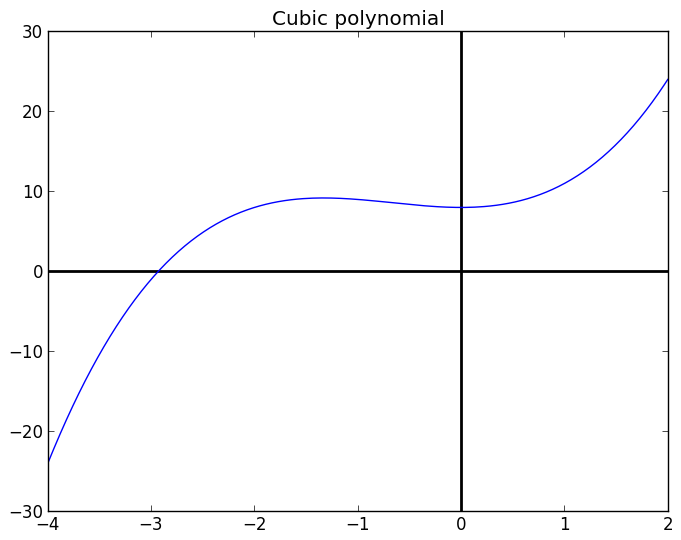
The plot reveals that this particular function only has one real root near -3. Let’s see if sympy can find all three roots for us.
In [361]: x = sym.Symbol('x')

# Syntax is expression that should be 0 and variable to solve for
In [362]: roots = sym.solve(x**3 + 2*x**2 + 8, x)

In [363]: print(roots)
[-2/3 - 4/(9*(-1/2 - sqrt(3)*I/2)*(4*sqrt(93)/9 + 116/27)**(1/3)) - (-1/2 - sqrt(3)*I/2)*(4*sqrt(93)/9 + 116/27)**(1/3), -2/3 - (-1/2 + sqrt(3)*I/2)*(4*sqrt(93)/9 + 116/27)**(1/3) - 4/(9*(-1/2 + sqrt(3)*I/2)*(4*sqrt(93)/9 + 116/27)**(1/3)), -(4*sqrt(93)/9 + 116/27)**(1/3) - 2/3 - 4/(9*(4*sqrt(93)/9 + 116/27)**(1/3))]

In [364]: pprint(roots)
                                                                      ________
                                                 /        ___  \     /     ___
   2                      4                      |  1   \/ 3 *I|    /  4*\/ 93
[- - - --------------------------------------- - |- - - -------|*3 /   -------
   3                          ________________   \  2      2   / \/       9
         /        ___  \     /     ____
         |  1   \/ 3 *I|    /  4*\/ 93    116
       9*|- - - -------|*3 /   -------- + ---
         \  2      2   / \/       9        27
________                             ________________
_               /        ___  \     /     ____
    116     2   |  1   \/ 3 *I|    /  4*\/ 93    116                       4
- + --- , - - - |- - + -------|*3 /   -------- + ---  - ----------------------
     27     3   \  2      2   / \/       9        27
                                                          /        ___  \
                                                          |  1   \/ 3 *I|    /
                                                        9*|- - + -------|*3 /
                                                          \  2      2   / \/
                          ________________
                         /     ____
                        /  4*\/ 93    116    2              4
-----------------, - 3 /   -------- + ---  - - - -----------------------]
 ________________    \/       9        27    3          ________________
/     ____                                             /     ____
  4*\/ 93    116                                      /  4*\/ 93    116
  -------- + ---                                 9*3 /   -------- + ---
     9        27                                   \/       9        27
If you parse through the printed items above you will see that sympy did find all 3 roots. Let’s ask sympy to give us the final answer with 5 significant digits.
In [365]: for i in range(len(roots)):
   .....:     print("Root %i = %s" % (i + 1, str(roots[i].n(5))))
   .....:
Root 1 = 0.46557 + 1.5851*I
Root 2 = 0.46557 - 1.5851*I
Root 3 = -2.9311
Just for fun let’s see if we can use scipy.optimize.fsolve to find the same roots:
In [366]: from scipy.optimize import fsolve

In [367]: def opt_func(x):
   .....:     return x**3 + 2*x**2 + 8
   .....:

In [368]: fsolve(opt_func, 0., full_output=1)
Out[368]:
(array([ 0.]),
 {'fjac': array([[-1.]]),
  'fvec': array([ 8.]),
  'nfev': 13,
  'qtf': array([-8.]),
  'r': array([  1.19165637e-07])},
 5,
 'The iteration is not making good progress, as measured by the \n  improvement from the last ten iterations.')

In [369]: fsolve(opt_func, -1., full_output=1)
Out[369]:
(array([ 0.00048317]),
 {'fjac': array([[-1.]]),
  'fvec': array([ 8.00000047]),
  'nfev': 29,
  'qtf': array([-8.00000047]),
  'r': array([  4.82322082e-05])},
 5,
 'The iteration is not making good progress, as measured by the \n  improvement from the last ten iterations.')

In [370]: fsolve(opt_func, -2., full_output=1)
Out[370]:
(array([-2.93114246]),
 {'fjac': array([[-1.]]),
  'fvec': array([  7.81597009e-14]),
  'nfev': 11,
  'qtf': array([  2.75358190e-08]),
  'r': array([-14.0501778])},
 1,
 'The solution converged.')
As you can see fsolve was able to find the correct real root, but it took a bit of work on our end to come up with a sufficiently good starting guess. It is also very important to note that we cannot solve for the imaginary roots using fsolve (or any other root finding routine in scipy) because the solutions form a hyperplane.
Application
We will use sympy to help us come up with an algorithm for quadratic extrapolation. One possible case where this could be useful is taking numerical derivatives on an evenly spaced grid. By the definition of the numerical derivative you will be unable to compute the derivative at the end point. One common technique used to do this is to use some sort of extrapolation to reach beyond the grid one point and use the extrapolated data to compute the derivative at the end points.
We will start with a generic quadratic polynomial.
In order to solve for the 3 coefficients \(a\), \(b\), and \(c\) we will need at least three data points: call them \((x_1, y_1)\), \((x_2, y_2)\), and \((x_3, y_3)\). To determine the constants, you set up three equations that force the parabloa to match the data points, like this:
with \(j = 1, 2, 3\), and then solve for \(a\), \(b\), and \(c\).
Todo
Assuming points \(x_1\), \(x_2\), and \(x_3\) are equally spaced with a separation of \(h\) (so that \(x_{j + 1} = x_j + h\)), solve the system of three quadratic equations for the parameters \(a\), \(b\), and \(c\) in terms of \(h\), \(x_1\), \(y_1\), \(y_2\), and \(y_3\). Hint: look at the sympy documentation for how to solve systems of equations.
Todo
Using the coefficients \(a\), \(b\), and \(c\) found in the previous problem, estimate the value of \(y(x)\) at three places in terms of \(y_1\), \(y_2\), and \(y_3\) (no \(x\) or \(h\) should appear in your solutions):
- At \(x _3 + h\) (one point beyond the grid)
- Half way between \(x_1\) and \(x_2\)
- Half way between \(x_2\) and \(x_3\).
Calculus
Derivatives
The derivative function in sympy can be accessed as an instance method for a sympy expression as in expr.diff(*vars). It can also be accessed as a function sympy.diff where the first argument is the expression as in sympy.diff(expr, *vars).
Notice the seemingly odd notation *vars. This was done intentionally to emphasize the flexibility provided by the diff function. *vars be best understood by example. In the following list we explore some of the things *vars can be. The syntax of the list is expr: what derivative operation is to take place.
- x: derivative with respect to x
- x, x, x: third derivative with respect to x
- x, 3: third derivative with respect to x
- x, y, x: derivative with respect to x, then y, then x again
- cos(x): derivative with respect to cos(x)
- x, 2, y, 2: second derivative with respect to x, then second derivative with respect to y
The general rule of thumb is that any combination of expressions or symbols can be used to specify the derivative operations. There are various subtleties associated with how sympy actually carries the operations out and in order to get a more complete understanding of them; see the documentation.
To demonstrate some of these derivative operations, we will use the expressions defined above.
In [371]: sym.pprint(ex_1)
   2            2
a*x  + a*x + b*x  - b*x + c

In [372]: sym.pprint(ex_2)
 3      2        2          2                  2    3      2          2    3
x  + 3*x *y + 3*x *z + 3*x*y  + 6*x*y*z + 3*x*z  + y  + 3*y *z + 3*y*z  + z

In [373]: sym.pprint(ex_3)
   2*x      2*x
a*e    + b*e

In [374]: sym.pprint(ex_1.diff(x))
2*a*x + a + 2*b*x - b

In [375]: sym.pprint(ex_1.diff(x, 2))
2*a + 2*b

In [376]: sym.pprint(ex_1.diff(x, x))
2*a + 2*b

In [377]: sym.pprint(ex_2.diff(x, y, z))
6

In [378]: sym.pprint(ex_2.diff(z, y, x))
6

In [379]: sym.pprint(sym.diff(ex_3, a, x, 4))
    2*x
16*e
Integrals
The integration functionality in sympy is also very powerful. sympy can provide definite and indefinite integrals for polynomial, rational, and exponential-polynomial. In addition, sympy can easily deal with integrals that, if they were to be solved by hand, would require multiple applications of integration by parts or u-substitutions.
Like the diff function, the integrate function can be accessed either as a method for an expression or as sympy.integrate. The call signature is a bit more simple for sympy.integrate, however, in that you need to give an expression and then one of two things:
- a variable of integration by itself
- a 3-element tuple (or list) (var, lower, upper), where lower and upper specify the lower and upper bounds of integration, respectively.
In [380]: sym.integrate(x**2, x)
Out[380]: x**3/3

# Notice the precision
In [381]: sym.integrate(x**2, (x, -2, 2))
Out[381]: 16/3

# Using method now
In [382]: ex_2.integrate(z)
Out[382]: z**4/4 + z**3*(x + y) + z**2*(3*x**2/2 + 3*x*y + 3*y**2/2) + z*(x**3 + 3*x**2*y + 3*x*y**2 + y**3)
Differential Equations
Dynamical systems are often represented as differential equations. sympy has robust support for the following types of ordinary differential equations (ODEs):
- 1st order separable differential equations
- 1st order differential equations whose coefficients or dx and dy are functions homogeneous of the same order.
- 1st order exact differential equations.
- 1st order linear differential equations
- 1st order Bernoulli differential equations.
- 2nd order Liouville differential equations.
- nth order linear homogeneous differential equation with constant coefficients.
- nth order linear inhomogeneous differential equation with constant coefficients using the method of undetermined coefficients.
- nth order linear inhomogeneous differential equation with constant coefficients using the method of variation of parameters.
In addition to ODE support, sympy can even solve separable (either multiplicative or additive) partial differential equations (PDEs).
The main functionality for ODE solving in sympy is the sympy.dsolve function. The call signature for this function is sympy.dsolve(eq, goal, **kwargs), where eq is the differential equation, goal is the function you want to end up with, and **kwargs is a placeholder for other arguments that could be passed to the function to help it out a bit. For more detail on what **kwargs could be, see the documentation. We will demonstrate its use by solving a simple differential equation:
In [383]: x, n = sym.symbols('x n')

In [384]: f = sym.Function('f')

In [385]: de = sym.diff(f(x), x, x) + 9*f(x)

In [386]: sym.pprint(de)
           2
          d
9*f(x) + ---(f(x))
           2
         dx

In [387]: soln = sym.dsolve(de, f(x))

In [388]: sym.pprint(soln)
f(x) = C1*sin(3*x) + C2*cos(3*x)
Application
Suppose you are given a set of demand functions.
where \(b < 0\) and \(c, g, h > 0\) are constants, \(Q_d, Q_s\) and \(P\) are the quantity demanded, quantity supplied and price, respectively. Also suppose that price is time varying and is a positive function of excess demand:
Todo
Use sympy.dsolve to solve the differential equation above.
Todo
Analyze the solution you just found by using values b, c, g, h, m = (-1.2, 2, 0.1, 1.1, 1.1). Solve for the constant of integration in two different cases by applying two different initial conditions \(P(0) = .5\) and \(P(0) = 1.3\), where t runs from 0 to 1. Plot the time series of prices. Hint: You should see that this economy is not very stable. Depending in the initial condition it will experience exponential growth or decay in prices.
Other
It is worth noting that sympy has the ability to do a lot more calculus based tasks such as:
- Limits
- Summations
- Series Expansions
- Special functions (Bessel, harmonic, spherical harmonic, gamma, zeta, factorials, polynomial families)
We will not cover these topics in detail here, but the excellent sympy documentation is a great place to start looking into these topics.
Linear Algebra
sympy also includes a Matrix class that can be used to perform symbolic linear algebra. There are a number of ways to instantiate an object of the sympy.Matrix class and we will show a few of them below.
# numpy-style. Specify lists of lists, one row at a time
In [389]: sym.Matrix([[1, 2], [2, 3]])
Out[389]:
[1, 2]
[2, 3]

# Using sym.eye, sym.ones, or sym.zeros
In [390]: sym.ones(2)  # Note one argument creates square matrix
Out[390]:
[1, 1]
[1, 1]

In [391]: sym.zeros((2, 4))
Out[391]:
[0, 0, 0, 0]
[0, 0, 0, 0]

In [392]: sym.eye(3)
Out[392]:
[1, 0, 0]
[0, 1, 0]
[0, 0, 1]

# Using a function to specify i, j entries
In [393]: def x_mat(i, j):
   .....:     return sym.Symbol('x%i%i' % (i, j))
   .....:

In [394]: sym.Matrix(4, 4, x_mat)  # give rows, cols, then function
Out[394]:
[x00, x01, x02, x03]
[x10, x11, x12, x13]
[x20, x21, x22, x23]
[x30, x31, x32, x33]
Accessing elements of a Matrix object is more similar to MATLAB syntax than numpy in that you can specify i, j pairs for a specific element, or give a single index and access the data as if it were a flattened list. Note that like in MATLAB or numpy, slices can be passed to get chunks of matrices at at time. See the examples for clarity.
In [395]: my_mat = sym.Matrix([[1, 2, 3], [4, 5, 6], [7, 8, 100]])

In [396]: my_mat
Out[396]:
[1, 2,   3]
[4, 5,   6]
[7, 8, 100]

In [397]: my_mat[3]
Out[397]: 4

# This should be the same as before
In [398]: my_mat[1, 0]
Out[398]: 4

In [399]: my_mat[1, 1:4]
Out[399]: [5, 6]
All standard matrix arithmetic works on Matrix objects. Note that unlike in numpy, the * operation does matrix multiplication, not element-wise multiplication.
There are many useful methods available to Matrix objects. Among them are:
|
|
|
Tips and Tricks
Printing Formats
All expressions or symbols in sympy can be represented in various formats. Among the more useful are sympy.latex(ex) and sympy.ccode(ex), which export the expression ex directly into latex format. This can be a big time saver, especially when working with matrices.
In [400]: print(sym.latex(my_mat))
\left[\begin{smallmatrix}1 & 2 & 3\\4 & 5 & 6\\7 & 8 & 100\end{smallmatrix}\right]

In [401]: print(sym.ccode(ex_2))
pow(x, 3) + 3*pow(x, 2)*y + 3*pow(x, 2)*z + 3*x*pow(y, 2) + 6*x*y*z + 3*x*pow(z, 2) + pow(y, 3) + 3*pow(y, 2)*z + 3*y*pow(z, 2) + pow(z, 3)
For more information on the printing capabilities of sympy see this page in the documentation.